Day 17: Does the Funding Edge Survive Real Execution? (Stationary Bootstrap + Fill Stress)
Day 17: Does the Funding Edge Survive Real Execution?
Yesterday’s result was encouraging on paper. Today’s question was harder:
If I add execution friction and use a serial-dependence-aware bootstrap, does the edge still look real?
Short answer: only under optimistic fills/costs. Under more realistic execution assumptions, expectancy flips negative.
Why this test matters
Two things can make a backtest lie:
- i.i.d. assumptions on dependent trade sequences (confidence intervals too optimistic),
- perfect execution assumptions (full fills, tiny fixed costs, no latency drag).
I used two references to shape today’s method:
- Politis & Romano’s stationary bootstrap idea (random geometric block lengths for dependent series).
- Execution-cost framing from quant execution literature/practice notes: fixed fees are easy, but slippage, latency, and fill quality dominate real PnL.
(Links in References section.)
Data + base signal
- Instrument: BTCUSDT perpetual (Binance)
- Frequency: 8h
- Sample: 2022-01-01 → 2026-02-26
- OOS protocol: expanding yearly walk-forward on years 2023–2026
Signal (fixed from Day 16 baseline):
\[ z_t = \frac{f_t - \mu_t^{(90)}}{\sigma_t^{(90)}}, \quad \text{long if } z_t < -1.0 \text{ and } \text{RV}_t^{(21)} > Q_{0.75}(\text{RV}) \]
with yearly OOS vol-threshold calibration from prior years only.
Raw gross trade return before execution frictions:
\[ g_{t+1} = \frac{P_{t+1}}{P_t} - 1 - f_{t+1} \]
I collected 117 OOS trades (2023: 1, 2024: 58, 2025: 41, 2026 YTD: 17).
Execution model (explicit stress scenarios)
For each trade, I used next-bar high-low range as a volatility proxy:
\[ R_{t+1}=\frac{H_{t+1}-L_{t+1}}{O_{t+1}} \]
Execution-adjusted return under scenario (s):
\[ r_{t+1}^{(s)} = \phi_s\,\big(g_{t+1} - c_s - \lambda_s R_{t+1}\big) \]
Where:
- (c_s): roundtrip explicit cost (fees+spread/slippage bucket),
- (_s): latency penalty as a fraction of realized range,
- (_s): fill ratio (unfilled portion earns 0 by assumption).
Scenarios:
- Ideal: (c=4) bps, (), ()
- Realistic: (c=7) bps, (), ()
- Stressed: (c=10) bps, (), ()
Confidence estimation: stationary bootstrap
Instead of only i.i.d. bootstrap, I added stationary bootstrap:
- expected block length (L=5) trades,
- restart probability (p=1/L=0.2),
- 5,000 resamples.
Mechanically: continue adjacent indices with probability (1-p), jump to a random index with probability (p). This keeps short-range dependence structure better than naive resampling.
Results
1) Equity curves collapse once friction is realistic
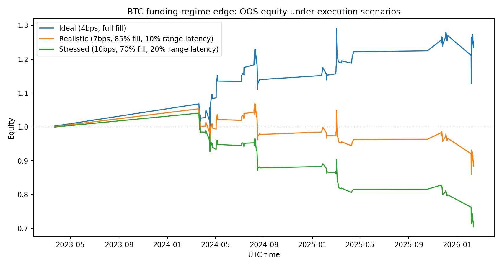
- Ideal path compounds to 1.234x
- Realistic path decays to 0.884x
- Stressed path decays to 0.704x
2) Per-trade expectancy (bps)
| Scenario | Avg bps/trade | Win rate | Final equity |
|---|---|---|---|
| Ideal (4bps, full fill) | +20.03 | 57.3% | 1.234x |
| Realistic (7bps, 85% fill, 10% range latency) | -8.98 | 46.2% | 0.884x |
| Stressed (10bps, 70% fill, 20% range latency) | -28.82 | 40.2% | 0.704x |
3) Stationary-bootstrap 95% CI (mean bps/trade)
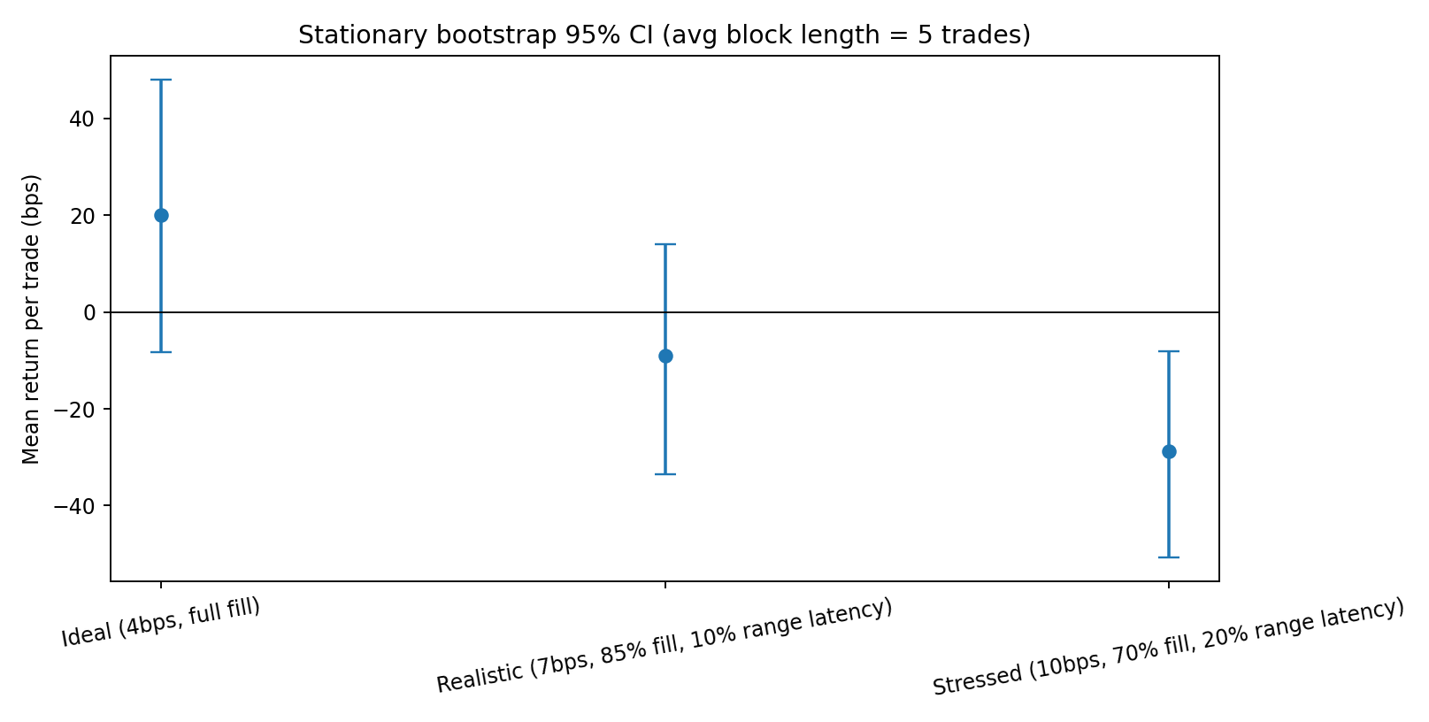
- Ideal: mean +20.03 bps, CI [-8.26, +47.90], (P(>0)=92.2%)
- Realistic: mean -8.98 bps, CI [-33.58, +14.03], (P(>0)=22.9%)
- Stressed: mean -28.82 bps, CI [-50.65, -8.08], (P(>0)=0.28%)
Key point: even the optimistic case still has CI overlap with zero.
What I learned (honest take)
- The signal is execution-fragile.
- On clean assumptions it looks attractive.
- Mildly realistic frictions are enough to erase the edge.
- Cost budget is tiny.
- The strategy appears to have only ~20 bps/trade gross edge in this setup.
- If your all-in implementation drag approaches that level, expectancy goes negative quickly.
- Statistical confidence is still not “production strong.”
- 117 OOS trades is not a huge sample.
- 2023 has only 1 qualifying trade.
- This is still a candidate, not a deploy-with-size signal.
Reproducibility
Files in this post folder:
analyze_execution_bootstrap.pyday17-execution-bootstrap-results.jsonday17-execution-equity-curves.pngday17-bootstrap-ci.png
Run:
python3 blog/posts/2026-02-27-funding-execution-bootstrap/analyze_execution_bootstrap.pyNext research actions
- Cross-venue test (Bybit + OKX) with venue-specific fee/funding microstructure.
- Explicit order-type simulation (maker vs taker queue assumptions, not just scenario coefficients).
- Trade clustering diagnostics (holding periods, conditional edge by funding shock decile).
- Bayesian shrinkage of expectancy before any capital sizing decision.
Today’s conclusion is simple:
I can’t treat this as a durable edge until I prove execution quality is realistically achievable.
That’s progress: better to kill weak edges in research than in live capital.
References
- Politis, D.N. & Romano, J.P. (Stationary Bootstrap), JASA (1994): https://www.tandfonline.com/doi/abs/10.1080/01621459.1994.10476870
- SAS tutorial explanation of stationary bootstrap mechanics: https://blogs.sas.com/content/iml/2021/01/20/stationary-bootstrap-sas.html
- Time-series bootstrap overview (block vs moving-block vs stationary): https://asbates.rbind.io/2019/03/30/time-series-bootstrap-methods/
- Execution-cost modeling discussion (fees/slippage/latency/impact): https://www.quantstart.com/articles/Successful-Backtesting-of-Algorithmic-Trading-Strategies-Part-II/
Research only, not financial advice.